IFMASS8

328 / 392

( )
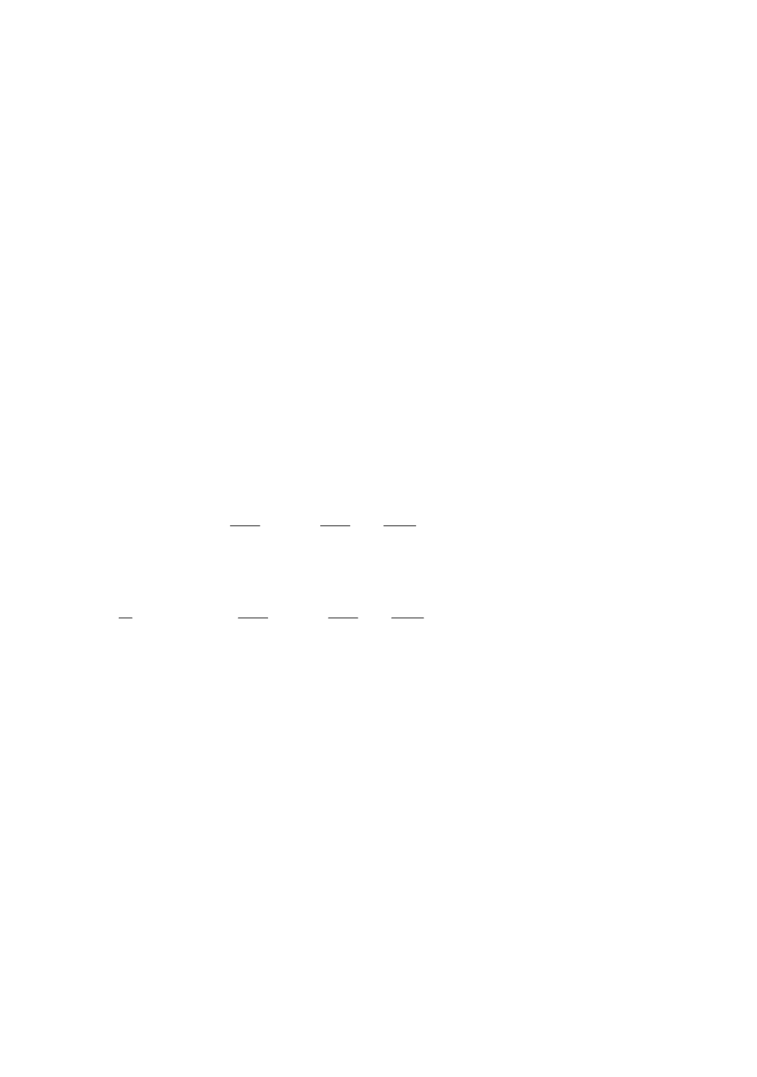
i ij j x X α θ = ( ) cos sin
sin cos ij
θ θ
α θ
θ θ
⎛ ⎞
= ⎜ ⎟
− ⎝ ⎠
, (12)
The same transformation also holds for the Jk integral [10], i.e.,
1
1
( ) cos sin
sin cos ( )
local
local
J
J
θ θ
θ θ
⎧ ⎫ ⎛ ⎞
= ⎨ ⎬ ⎜ ⎟
−
⎝ ⎠ ⎩ ⎭
(13)
For sake of numerical implementation and computational efficiency within the FEM,
Eq. (10) is evaluated in global coordinates.
When the material of the considered structure is homogeneous and body forces are
absent, the finite element implementation of Eq. (10) becomes very similar to that of the
contour integral. The only difference is the introduction of the weight function q, when
Eq. (10) is used. With the isoparametric finite element formulation, the distribution of q
within the elements is determined by a standard interpolation scheme with use of shape
functions hi:
1
m
i i
i
q h Q
=
= ∑ (14)
where Q i are values of the weight function at nodal points, and m is the number of nodes.
Spatial derivatives of q can be found by usual procedures for isoparametric elements.
The equivalent domain integral in 2D can be calculated as a sum of discretized values
of Eqs. (10) and (11), [5]:
elements 1
in
det
P
i
k ij kj
p k j n p
A
u X qm
p J W w
X X
σ δ
η
=
⎡ ⎤ ⎛ ⎞ ⎛ ∂ ∂ ∂
= − ⎢ ⎜ ⎟ ⎜
∂ ∂ ∂
⎢⎝ ⎠ ⎝ ⎣ ⎦
∑ ∑
⎞
⎥⎟
⎥⎠
i, j,k,m ,n = 1,2 (15)
and the equivalent domain integral in 3D [5,7] is
elements 1
in
1 det
P i
k ij kj
p k j n p
V
u X qm
p J W w
f X X σ δ η
=
⎡ ⎤ ⎛ ⎞ ⎛ ∂ ∂ ∂
= − ⎢ ⎜ ⎟ ⎜
∂ ∂ ∂
⎢⎝ ⎠ ⎝ ⎣ ⎦
∑ ∑
⎞
⎥⎟
⎥⎠
i, j, k,m,n = 1,3 (16)
The terms within [·]p are evaluated at Gauss points with use of Gauss weight factors,
for each point, wp. The present formulation is for a structure of homogeneous material in
which no body forces are present. For the numerical evaluation of the above integral, the
domain A is set from the set of elements about the crack tip. The domain A is set to
contain all elements which have a node within a sphere of radius rd about the crack tip.
Figure 3 shows a typical set of elements for domain A. This figure shows the contour plot
of the weight function q for the elements. The function q is then easily interpolated within
the elements using the nodal shape functions, according to Eq. (14).
Function q(x) can be interpreted as a rigid translation of nodes inside Γ, while nodes
on Γ remain fixed. The set of nodes moved rigidly is referred to as the rigid region, and
the function q(x) as the shift function. PAK allows an automatic search for nodes of the
rigid region. The first region consists of nodes of all elements connected to the crack tip
node, i.e., rd = max(∆ x,∆y ), where (∆x, ∆y) is the length of an element with crack tip. The
second region or ring consists of all nodes in the first region and nodes of all elements
connected to any node in the first region, i.e. rd = 2max(∆x,∆y). Therefore, the contours of
larger size domain are determined.
324