


 318 / 392

with
0.2
0.001
min
0.6
p
E R
µ
⎧⎪
=
⎨
⎪⎩
(16)
and
( 1) 2
( )
(
1)
N
r
r
r
f L f L L
−
= =
N
for 1 ≤
L
r
<
L
r max
(17)
0.2
0.3 1
p
m
R
N
R
⎡
⎤
= −
⎢
⎥
⎣
⎦
(18)
0.2
0.2
1
2
p
m
r max
p
R R
L
R
⎡
⎤
+
=
⎢
⎥
⎢
⎥
⎣
⎦
(19)
with
L
r max
being the limit against plastic collapse.
– Advanced Level
1 2
2
1
( )
2 (
)
ref
r
r
ref
ref
ref
E
L
f L
E
ε
σ
ε
σ
−
⎡
⎤
=
+
⎢
⎥
⎢
⎥
⎣
⎦
for 0 ≤
L
r
≤
L
r max
(20)
f
r max
Y
L
σ
σ
=
with
1 (
)
2
f
Y m
R
σ
σ
= +
(21)
Different to the Levels above,
f
(
L
r
) is a continuous function which follows the true
stress–strain curve in a point-wise manner. Each value of
σ
ref
is assigned to an
L
r
value by
ref
r Y
L
σ
σ
=
(22)
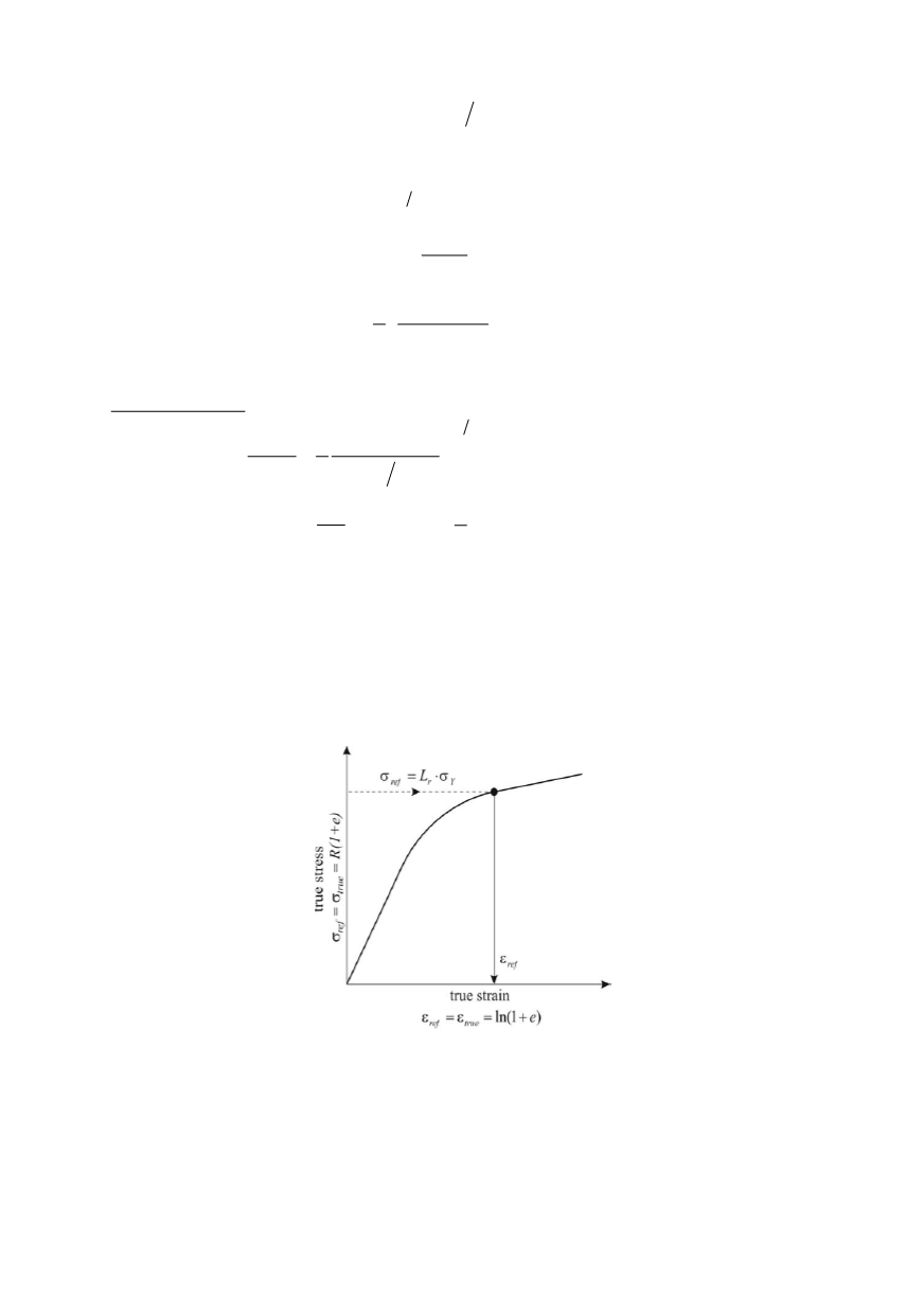
The corresponding reference strain
ε
ref
is obtained from the true stress–strain curve as
illustrated in Fig. 14. No distinction is necessary between materials with and without a
Lüders plateau. On the other hand
σ
ref
/
ε
ref
values have to be available at
L
r
= 0.7/0.9/0.98/
1/1.02/1.1, and other values of
L
r
.
Figure 14. True stress and strain in terms of the loading parameter,
L
r
1.8. The true stress–strain curve of the material
The engineering stress–strain curve of the material is shown in Fig. 15. Five tests were
carried out but only the lowest curve was used for SINTAP analysis. The mechanical
properties derived from these curves are summarized in Table 1. With
σ
and
ε
designat-
ing the engineering stress and strain, the true stress and strain values,
σ
t
and
ε
t
are deter-
mined by
314