


 352 / 392

348
0.5)
N
1 1(0.5)
m
m
D D N
N
N
σ
σ
=
;
1
1(
log log
log
log
D
D
N
m
N m
σ
σ
+
=
+
6
6
1(0.5)
1
log(
) log(0.095 10 2.5 10 ) 12.43
log(
)
log(748 973)
D
D N
N N
m
σ σ
⋅
⋅
=
=
=
It is possible to calculate in the same way the exponents,
m
, for border lines for proba-
bilities
P
R
= 0.1 and 0.9. They differ little from the value of this exponent for
P
R
= 0.5 as
the dissipation range spreads gradually from higher to lower stresses. In absence of more
precise information it is possible to take that lines for
P
R
= 0.1, 0.5, and 0.9 are mutually
parallel, and that exponents
m
are mutually equal.
The infinite fatigue life strength is reduced with the reduction of material strength,
also with increase of structural non-homogeneity, and with increase of stress concentra-
tion, etc. With reduction of infinite fatigue life strength (endurance limit) with respect to
static strength, the exponent
m
decreases. If the endurance limit is increased by surface
reinforcement and if it approaches static strength, the exponent
m
increases (as in the
indicated example). The infinite life limit
N
D
may be decreased with decrease of
σ
D
, but
more often it stays the same.
7. FAILURE PROBABILITY FOR SERVICE FATIGUE STRENGTH
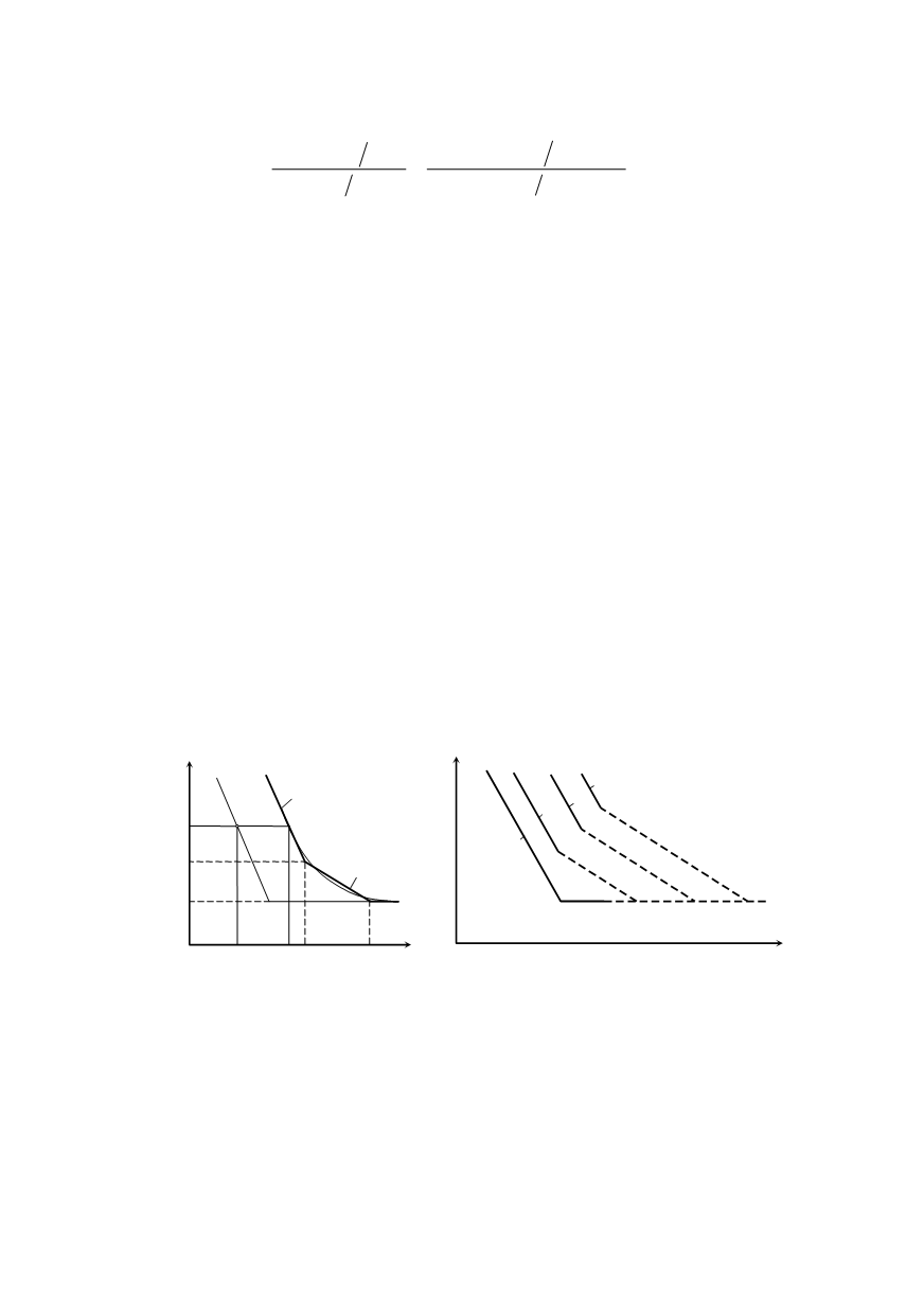
The service fatigue strength
σ
R
follows the curve in the double logarithmic coordinate
system (Fig. 16a). By approximating this slightly curved line with a broken up straight
line, a line is obtained with two breaking points, the coordinates of which are presented in
the figure as equations of the parts of these lines. The coordinates of the breaking point
σ
R0
,
N
R0
and the exponent
q
are parameters of the service fatigue strength curve. The
position of the curve in the coordinate system depends on the weight of the work regime.
In case of the light one (
l
), the curve is shifted to the right, i.e. towards the range of
extremely high numbers of cycles up to fracture
N
R
. With an increase of the heaviness of
the regime, the service fatigue strength curve approaches the Wöhler’s (
w
).
log
σ
log
N
w
h m l
a)
b)
R R
q
R
C N
=
σ
log
σ
N
log
σ
R
σ
R
=
σ
σ
R
σ
D
N
1
N
N
R
N
RD
log
N
R R
m
R
C N
=
σ
Figure 16. Service fatigue strength curves: a) approximation by broken straight line; b) the impact
of the heaviness of work regime onto the relation of the curve of service and basic strength
The testing of service fatigue strength and failure probability for service fatigue
strength is quite complex in comparison with this testing of basic strength. Two basic
additional problems are imposed here. One relates to the manner of creating loads (stress)
in the course of testing, the other relates to the choice of stress level for testing. The stress
spectrum is an ordered set of stress changes. By ordering this set, the sequence has been
lost and the impact of small and big changes has been mixed up. Gassner has suggested a
solution for this problem. Following his suggestion, the ordered set should be mixed
again so that the simulation effect is as close as possible to the effect of real random