


 351 / 392

23
760
( ) 1
N
N
P
e
σ
σ
⎛ ⎞
−
⎜ ⎟
⎝ ⎠
= −
In the absence of more precise information, this function of distribution of failure proba-
bilities may be valid for all cycle numbers which are greater than infinite life limit
N
D
.
6. THE FIELD OF THE BASIC FATIGUE STRENGTH DISSIPATION
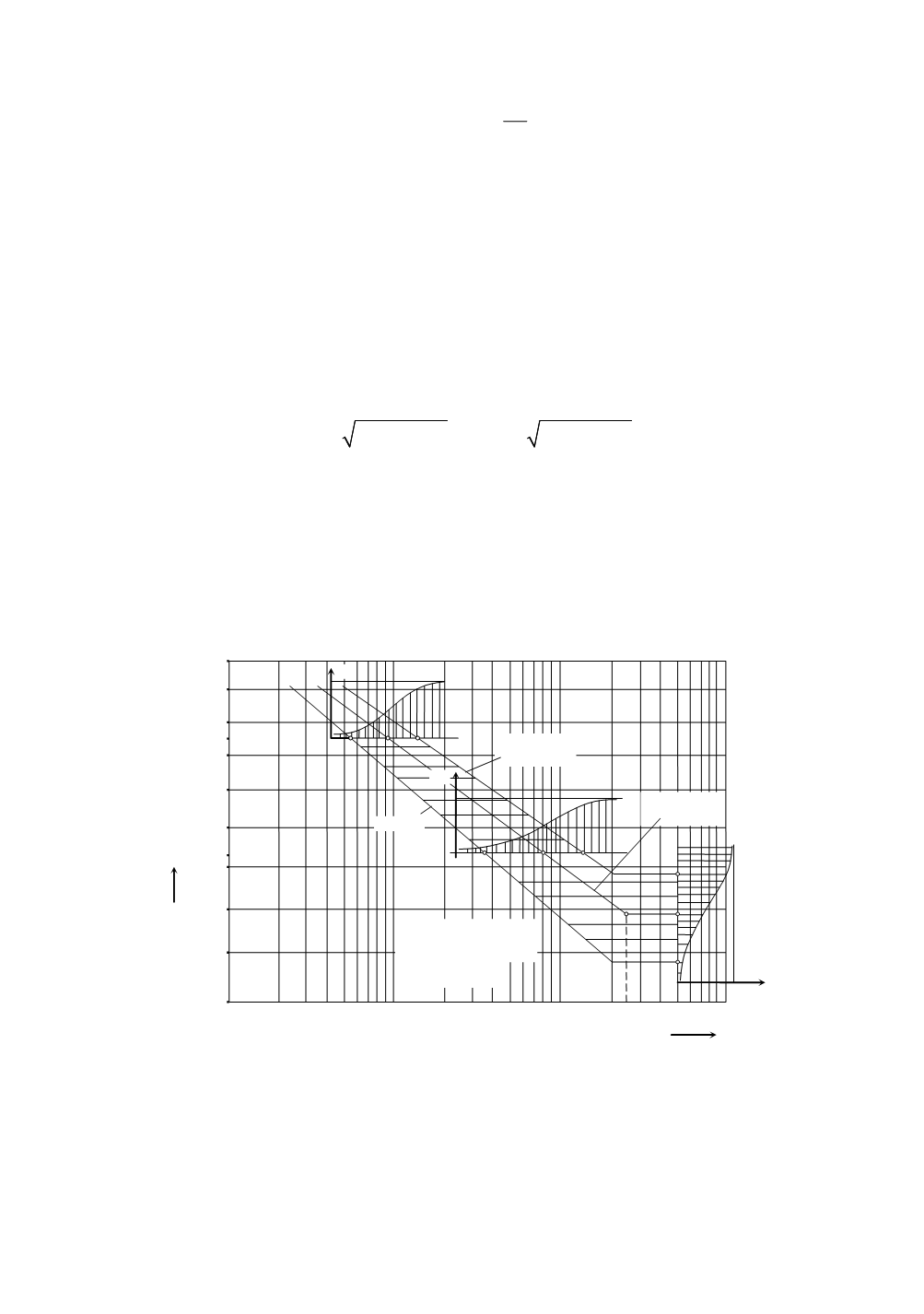
It is possible to form the field of fatigue strength dissipation by using functions of
failure probability obtained by testing two stress levels in the range of finite-life strength
and for the infinite-fatigue-life. That field covers all stress levels and numbers of cycles.
This range is by rule limited by lines with failure probabilities
P
R
= 0.1 and 0.9, and the
line with failure probability
P
R
= 0.5 is most frequently in use. By using the indicated
three distributions of failure probability, it is possible to calculate cycle numbers, i.e.
stresses which correspond to the indicated probabilities and that means
ln(1 )
R
N
P
β
η
= − −
;
ln(1 )
N
R
P
β
σ
η
= − −
with the use of respective parameters
η
and
β
. In this way points are determined for stress
levels
σ
N
1
and
σ
N
2
and for the number of stress cycles
N
DV
. The calculated coordinates
have been entered into the coordinate system with logarithmic axes, Fig. 15. By joining
the points with the same probability
P
R
, border curves are obtained
P
R
= 0.1,
P
R
= 0.9 as
well as the middle line for
P
R
= 0.5. The failure probability distributions have been pre-
sented on stress levels
σ
N
1
= 973 N/mm
2
,
σ
N
2
= 810 N/mm
2
and for
N
DV
= 5·10
6
. Based on
border lines, it is possible to define distributions for any stress
σ
N
and for any number of
stress cycles
N
.
1100
1050
1000
950
900
850
800
750
700
10
4
10
5
10
6
10
7
N
D
N
σ
N
N/mm
2
σ
N
1
σ
N
2
P
R
P
R
=0,1
P
R
P
R
0
1
0
1
1
P
R
=0,
P
R
=0,
σ
D
=748N/m
2
N
D
=2,5
⋅
10
6
12
Figure 15. Dissipation field of failure probabilities for basic fatigue strength
The middle line in the dissipation field, for failure probability
P
R
= 0.5 represents
Wöhler’s
S
–
N
curve. It is defined by three parameters
σ
D
(
σ
lim
),
N
D
and
m
. The coordi-
nates of breaking point are
σ
D
=
σ
lim
= 748 N/mm
2
and
N
D
= 2.5·10
6
and are defined by
reading from the diagram. The exponent by which the inclination of Wöhler’s curve is
defined is obtained on the basis of coordinates of points on this line, i.e.
347