


 349 / 392

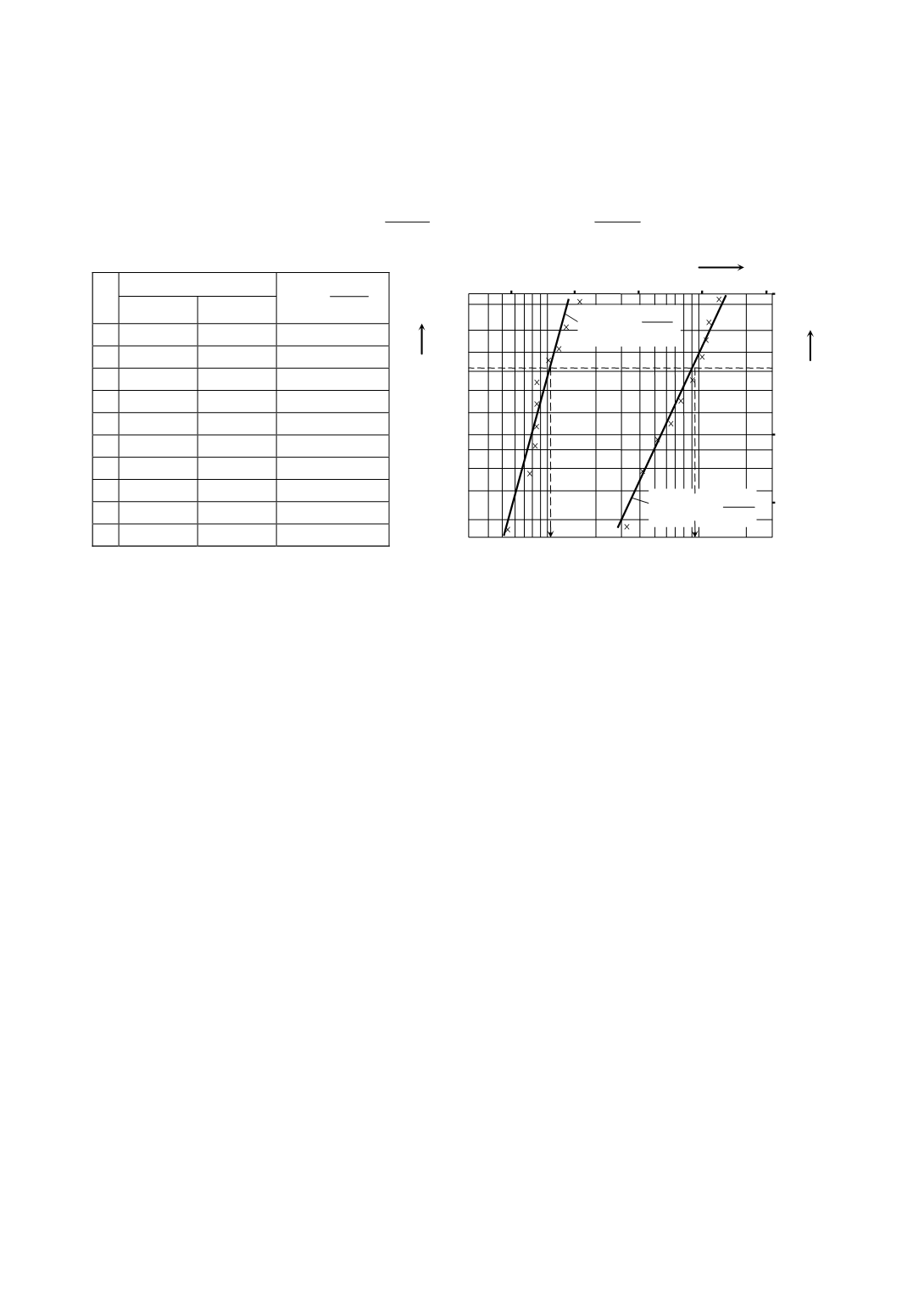
following the methodology, presented in Section 2. The obtained values of parameters for
stress
σ
N
1
= 973 N/mm
2
are
η
= 105 000 cycles,
β
= 3.8 and for stress
σ
N
2
= 810 N/mm
2
,
η
= 950 000 cycles,
β
= 2.6. For these parameters and for respective stress levels of
Weibull’s distribution, the failure probabilities are
3.8
105000
( ) 1
N
R
P N e
⎛
⎞
−
⎜
⎟
⎝
⎠
= −
;
2.6
950000
( ) 1
N
R
P N e
⎛
⎞
−
⎜
⎟
⎝
⎠
= −
345
0,2
4 6 8
10
5
2 3 4 6 8
10
6
-2
-1
0
1
P
R
x
=ln
N
Y
0,9
0,8
0,7
0,6
0,5
0,4
0,3
0,1
11
12
13
14
15
σ
N
N
m
m
2
97
=
2
σ
N
N
m
2
81
=
N
N
for
σ
N
in N/mm
2
z
i
σ
N
1
= 973
σ
N
1
= 810
1
i
R
z
P
z
Σ
=
+
1 52380 331500
0.091
2 76800 419800
0.182
3 82315 512320
0.273
4 82530 650030
0.364
5 87820 768000
0.455
6 89930 905320
0.545
7 102415 102865
0.636
8 123300 113460
0.727
9 131050 121350
0.818
10 175200 1383000 0.909
Figure 12. Distribution of failure probability in the range of finite life strength
5. FAILURE PROBABILITY IN THE RANGE OF INFINITE–LIFE STRENGTH
In the range of the infinite–life strength, the distribution of failure probability is
defined for a fixed stress cycles number up to fracture, and the independent variable is
stress, i.e. fatigue strength
σ
N
. The realization of the test process of this probability is pre-
ceded by the decision making about the fixed number of stress cycles up to which the
tests are to be conducted, as well as the decision about the stress level number for which
sets of
z
Σ
specimens (parts) are to be tested. The stress cycle number up to which the
specimens are tested is a post infinite life limit number of cycles
N
DV
. That is the number
of stress cycles for which it is known for sure that it is greater than the infinite life limit
N
D
, but it is not too large, so that tests should not become too long-lasting. The test speci-
mens which fracture at the number of cycles
N
<
N
DV
are classified as failed test speci-
mens’
z
i
at a respective stress value (level), and those that do not fail up to
N
DV
are
classified in the group that have not failed
z
Σ
–
z
i
. At higher stress levels (closer to finite-
life strength) of the same number of test samples
z
Σ
, there is a greater number of failed
samples
z
i
. With decrease of the stress level there is a decrease in the number of failed
specimens, and the number of specimens that endure the
N
DV
cycles increases.
The problem of stress level selection is more complex. The decision is made about the
number of stress levels, their density, and stress values. If the value of the endurance limit
σ
D
(
σ
lim
) and the value of the dissipation range are known, several stress levels are uni-
formly distributed in that range, such as for example
σ
N3
,
σ
N4
,
σ
N5
,
σ
Nk
(Fig. 13a). This is
the stress level method, following which further tests take place on
z
Σ
specimens and the
calculation of the failure probability
P
R
=
z
i
/(
z
Σ
+ 1)
.
If the value of infinite-life strength is
not known in advance, the level method cannot be applied, i.e. this method must be
preceded by application of the step method. Following the step method, after each tested
specimen the stress level changes, with which the next specimens will be tested. If a test