


 343 / 392

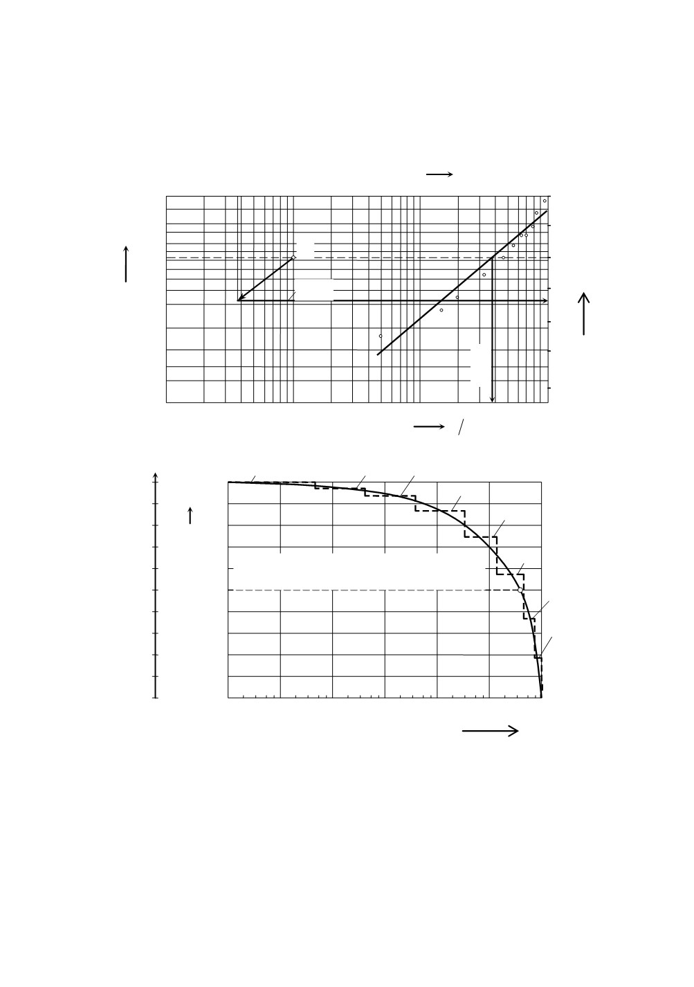
units on the logarithmic axis with the scale from 100 to 106 stress cycles (Fig. 8). With
this transformation the cumulative function
F
(
σ
a
) has been translated into the logarithmic
form, where the range of large stress amplitudes has been spread out onto about 2/3 of the
horizontal axis, and the field of small and medium stress amplitudes has been compressed
onto 1/3.
0.1
0.2 0.3
1 2
3 4 5 10 20 30 50 100
0,99
0,95
0,80
0,60
0,40
0,30
0,20
0,10
0,05
0,03
0,02
0,01
-2
-1
0
1
2
3
4
0
-1
-2
-3
-4
+1
+2
β
=1.3
η
=38
σ
a
N mm
2
C
X=
ln
σ
a
Y
F(
σ
a
)
Figure 7. Parameters of Weibull’s function determination for stress amplitude distribution
x
1,0
100
1
2
3
0,5
0
σ
a
N/mm
2
60
0
20
40
80
4
5
6
7
8
10
0
10
1
10
2
10
3
10
4
10
5
10
6
2 4
6 8 2 4 6 8 2 4 6 8 2 4 6 8 2 4 6 8 2 4
6 8
( )
(
)
62,5 10 42,0 log
log
6
= ⋅
=
b a
n H
σ
n
b
Figure 8. Logarithmic presentation of the stress spectrum
The continuous shape of the logarithmic curve is not suitable for use in calculations or
for endurance testing. The step-like shape is more suitable for this purpose. The optimal
number of steps (stress levels) is eight. The division is formed by forming more steps in
the range of greater values of stress amplitudes (differences in stress levels are smaller),
and in the range of smaller amplitudes there are less steps with greater differences in
level. After the division it is possible to create a tabular form, i.e. a table filled up with
values which are read from the graphical presentation (Fig. 8).
339