


 342 / 392

where the independent variable
x
is substituted by the stress amplitude
σ
a
. The parameters
of this distribution are
η
and
β
, which may be determined in the simplest way by graphi-
cal method. It is necessary to transform Weibull’s function into the form of a straight line
for this purpose. This is achieved by double logarithm of the transformed form of
Weibull’s function
( ) 1
x
F x
e
β
η
⎛ ⎞
−
⎜ ⎟
⎝ ⎠
= −
, i.e. ( ) 1
a
a
F
e
β
σ
η
σ
⎛ ⎞
−
⎜ ⎟
⎝ ⎠
= −
1
ln ln
ln
ln
ln
1 ( )
a
a
a
F
β
σ
β σ
β η
σ
η
⎛ ⎞
=
=
−
⎜ ⎟
−
⎝ ⎠
and substitution
1
ln ln
1 ( )
a
F
σ
=
−
ln
a
X
σ
=
Y
;
;
a
β
=
;
ln
b
β η
= −
from where it follows that
Y
=
aX
+
b
is the equation of the straight line in the coordinate
system with the respective logarithmic scale.
0,2
0,4
0,6
0,8
1,0
0
20 40 60 80 100
f
i
F
i
0,2
0,4
0,6
0,8
1,0
0 20 40 60 80 100
σ
a
N mm
2
σ
a
N mm
2
a)
b)
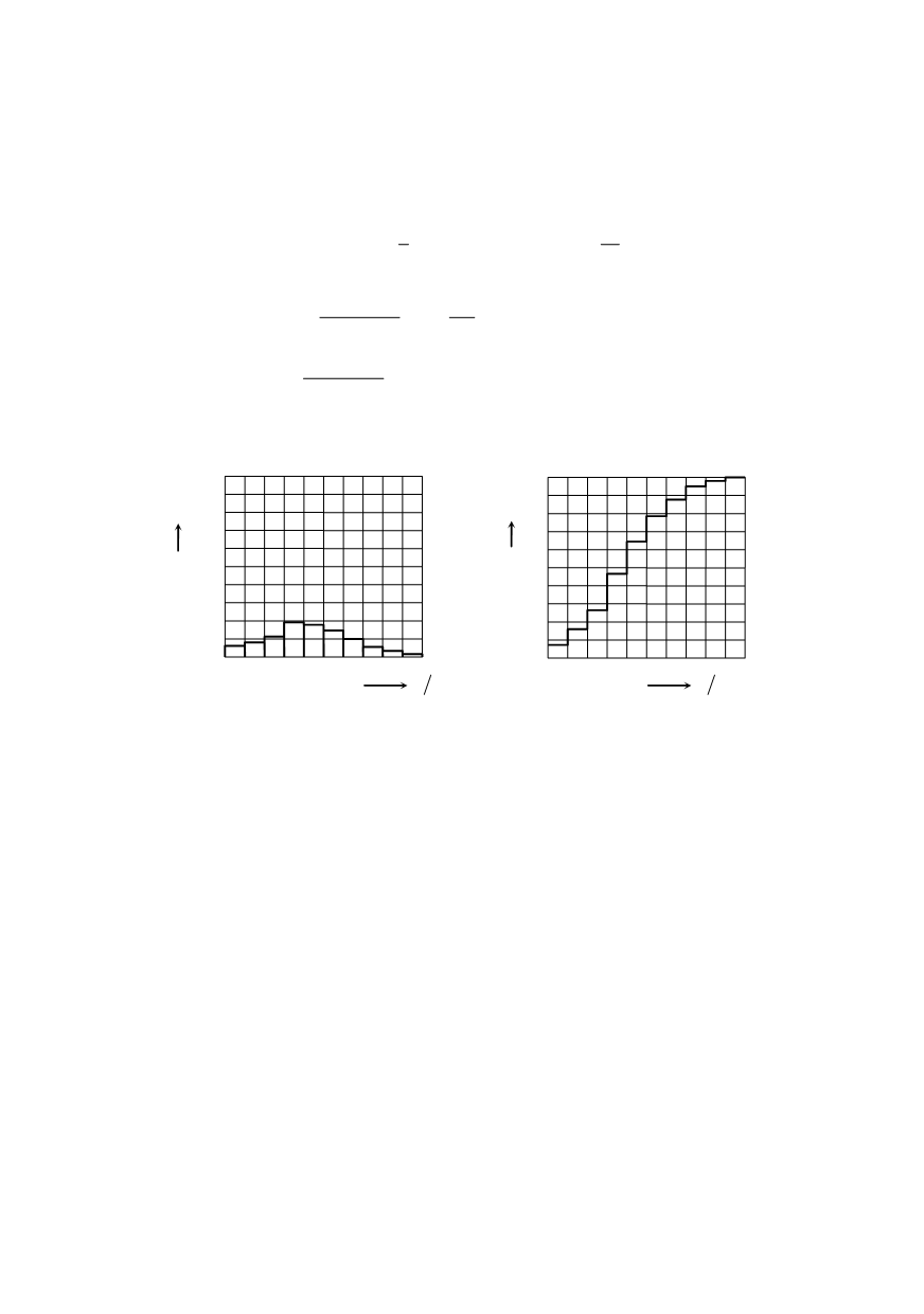
Figure 6. Histograms of the probability density and the cumulative function
Figure 7 shows the coordinate system with uniform scale on the coordinates
X
and
Y
(upper and right scale). Starting from expressions for
X
= ln
σ
a
and
Y
= lnln{l/
[
l –
F
(
σ
a
)
]
}
and from this uniform scale, values have been calculated for
σ
a
and for
F
(
σ
a
), the values
of which are given on the lower and left scale. This is how the Weibull’s coordinate
system is obtained. Experimental (empirical) values of cumulative probability
F
(
σ
a
) are
entered for each class of stress amplitudes
σ
a
. A series of points is obtained which follow
closely the straight line. After entering, this set of points is approximated by a straight
line. Coordinates
X
and
Y
enable determination of parameters in the equation of the
straight line,
a
and
b
, and thereby also the parameters of Weibull’s distribution,
η
and
β
.
After approximating experimental points by a straight line, the parameter
η
expressed in
the stress units is read in the intersection of the straight line with the
X
axis, i.e. that is the
stress value for the probability
F
(
σ
a
) = 0.632. Dimensions of parameter
η
are same as
σ
a
,
thus in expression
F
(
σ
a
) the ratio
σ
a
/
η
is a dimensionless value. Parameter
β
= 1.3 is the
part on the
Y
axis for
∆
X
= 1 and represents a dimensionless value.
338
The greatest stress fluctuations have the greatest effect on fatigue of the material. The
number of their occurrences, i.e., the frequency of occurrence is small. In this sense, a
more correct and clear presentation offers the logarithmic form of the cumulative function
shown in Fig. 8. The values of function
H
(
σ
a
) = 1 –
F
(
σ
a
) = 1...0 are multiplied with a
suitable number of stress cycles
n
b
= 106. The multiples are logarithmic for each value
σ
a
and values log(
H
(
σ
a
)
n
b
) are obtained between 1...6. This is the number of the logarithmic