IFMASS8

341 / 392

2. STRESS SPECTRUMS AND EXPLOITATION REGIMES
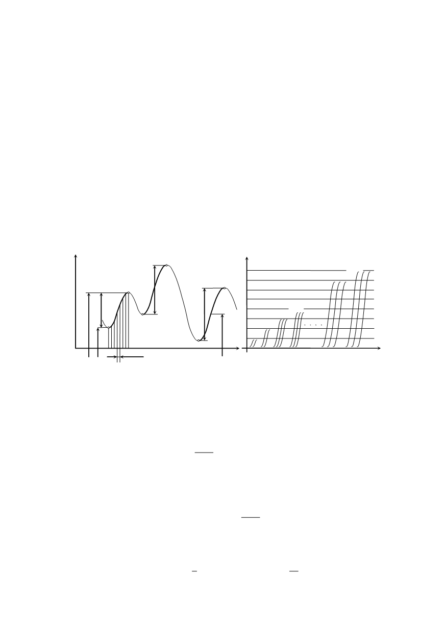
Figure 5 shows the possible analogous random function of stress fluctuation with
marked values of change, i.e. stress change ranges σs = 2 σa , where σa is the stress ampli-
tude. The mean values σm around which stress fluctuates, are also variable. It is necessary
to make a selection of values of the changes and their mean values, classify them into
classes and determine the number of occurrences of each of the values of changes. If the
analogous (uninterrupted) time function is digitalized, it transforms into a set of numeri-
cal values in small time intervals ∆t, as presented in Fig. 5a. The program for processing
digital values compares each one of them with the previous one and determines the values
of neighbouring extremes – minimum and maximum, and calculates the spans σsi =
σmaxi – σmini . The span is calculated only at the increase of stress so that the cycles are not
doubled. The calculated spans can be classified by their value and by mean stress values.
For the purpose of simplification, further analysis relates only to spans. Figure 5b shows
that the calculated values of the spans are classified in certain classes – fields of equal
value. For example, the first class, for i = 1, would include all spans σsi = 0...20 N/mm2,
and the second for i = 2 would include spans σs2 = 20...40 N/mm2, and the third for i = 3,
σs3 = 40...60 N/mm2 etc.
σ
σmax
σm
σs
σs
σs
σm
∆t t
∆nu 2
∆nu i
∆nu k
a) b)
Figure 5. Processing (classification) of the stress amplitudes
Statistical processing of obtained results of stress spans (amplitude) classification
consists of determining the rule by which their values behave. If stress classes are marked
by i = 1,2,3...k and if in each class there is a ∆nu1, ∆nu 2,...∆nuk, the span occurrence σs 1,
σs2,... σsk, i.e. amplitude σa1, σa2,... σak, the frequency of occurrence of each class is
ui
i
u
n f
n
∆
= ;
1
k
u u
i
n n
=
= ∆∑ i
In the graphical form the frequency of the occurrence of stress classes represents a
histogram of probability density (Fig. 6a) which may transform into a histogram of
cumulative probability (Fig. 6b), following the expression
1 1
k k ui
i i
i i u
n
F f
n
= =
∆
= =∑ ∑
These empirical values are translated in the most efficient manner into an analytical
form by using Weibull’s function
( ) 1
x
F x e
β
η
⎛ ⎞
−⎜ ⎟
⎝ ⎠ = − , i.e. ( ) 1
a
a F e
β
σ
η
σ
⎛ ⎞
−⎜ ⎟
⎝ ⎠ = −
337