
316
0
f
f
S
K K
σ
− =
(22)
One needs to evaluate both terms in Eq. (22), using a procedure similar to the one used
in previous section for the averages. Now the following scheme is applied
i
i
0
0
0
0
1/2
2
,
0
1/2
2
,
0
1
( , , )
1
( , , )
c a
f
f
c c a
c
c a
f
f
S
S
S
c c a
c
K K
K c R dc
a
K K
K c R dc
a
σ
σ
σ
α
α
+
+
+
+
⎧
⎫
⎪
⎪
⎡
⎤
→
= ⎨
⎬
⎣
⎦
⎪
⎪
⎩
⎭
⎧
⎫
⎪
⎪
⎡
⎤
→
= ⎨
⎬
⎣
⎦
⎪
⎪
⎩
⎭
∫
∫
(23)
The resulting functions depend on the fractal exponent
α
and two length-like variables
X
and
R
. To calculate the
K
-factors for a fractal crack the expression given by Wnuk and
Yavari /27 allows to obtain
1
2
2
2 1/2
2 2
0
(
)
(
)
( )
a
f
a
a x
a x
K
p x dx
a x
α
α
α
σ
α
π
−
−
+ + −
=
−
∫
(24)
In the first equation in (23) the substituting
σ
for
p
(
x
) and
c
+
R
for
a
leads to
( , , )
( )
(
)
f
K c R
c R
α
σ
α
χ α σ π
=
+
(25)
The scalar function appearing in this equation reads
2
2
1
2
2
0
1 (1 ) (1 )
( )
(1 )
s
s ds
s
α
α
α
α
χ α
π
+
−
=
−
∫
(26)
Next evaluation of the average produces
0
1/2
1/2
1
2
2
2
2
0
0
0
1
( )
(
)
( )
( '
)
'
c a
X
f
c
X
K
a
c R dc
a
X R dX
a
α
α
α
α
σ
χ α σ π
χ α σ π
+
+
⎧
⎫
⎧
⎫
⎪
⎪
=
+
=
+
⎨
⎬
⎨
⎬
⎪
⎪
⎩
⎭
⎩
⎭
∫
∫
(27)
The integral is elementary and one can obtain
1/2
2 1
2 1
2
0
(
1)
(
)
( )
2 1
f
X R
X R
K
a
α
α
α
σ
χ α σ π
α
+
+
⎡
⎤
+ +
− +
⎣
⎦
=
+
(28)
It is readily observed that for the fractal dimension
1
D
→
(or
1/ 2
α
→
) expression
(28) reduces to the equation valid for non-fractal discretized cohesive model
1/2
0
1
2
K
a X R
σ
σ π
⎛
⎞
=
+ +
⎜
⎟
⎝
⎠
(29)
Let us define the ratio of the last two
K
-factors
1/2
0
( , , )
f
f
K
k
a
X R
K
σ
α
σ
σ
σ
χ
α
−
=
=
(30)
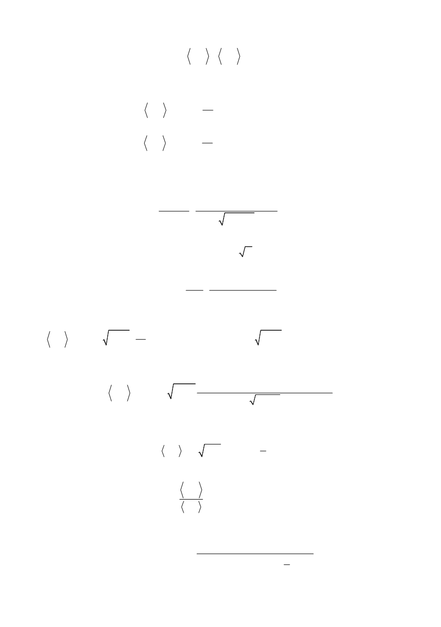
where the new scalar function is defined as follows
1/2
2 1
2 1
(
1)
(
)
( , , )
( )
1
(2 1)(
)
2
X R
X R
X R
X R
α
α
σ
χ
α
χ α
α
+
+
⎡
⎤
⎢
⎥
+ +
− +
=
⎢
⎥
⎢
⎥
+ + +
⎣
⎦
(31)


