IFMASS10

53 / 352

49
hardening curve (i.e. “universal” flow curve) ߪത ൌ ݂ሺߝ ҧሻ. Time rate of actual stress is
singled out by the requirement that it must be compatible with the current rate of strain
hardening, by tangent to the strain hardening curve. It must be noted that this statement
does not hold for arbitrary assumed or virtual deviatoric stresses and strains, Tᇱ and ߝ ᇱ .
This assumption implicitly states that actual and virtual stress and strain coincide until
actual instant of time (denoted by ߬ ൌ 0). Then these two may split such that actual stress
increment remains tangent to actual stress trajectory, whereas virtual stress may be
oblique with respect to it. If the condition of Eq. ( 14 ) is not satisfied, then bifurcation
leading to plastic instability takes place.
A2-3. The strain tensor used almost exclusively by Hill /29/ is logarithmic Eulerian
(true) strain tensor which in terms of its proper directions iԦଵ, iԦଶ, i Ԧଷ has the form (with
summation over repeated indices implied), ߝ ൌ iԦ௞۪i Ԧ௞ ln ߣ௞ ؠ iԦ௞ ۪iԦ௞ߝ௞, where ߣଵߣ ,ଶ ߣ ,ଷ
are principal stretches. For a parallelepiped with edges L1, L2, L3 is ߣ௞ ൌ L௞ L
଴௞ ⁄
ሺ݇ ൌ 1,2,3ሻ. The conjugate stress tensor is Cauchy stress such that work increment
equalsߜ ܹ ൌ T :δε. According to this assumption ߝݎݐ ൌ 0, ߝݎݐ ሶ ൌ 0 for advanced plastic
strains. This means that elastic strains are negligible and plastic incompressibility holds.
A2-4. For proportional plane stress paths ݉ ൌ ߪଶ ߪଵ ൌ ܿ݋݊ݐݏ ⁄ the onset of diffuse
instability appears when ߪሶ
ଵ ߪଵ ൌ ߝ ሶ
ଵߪ ,ሶ
ଶ ߪଶ ൌ ߝሶ
ଶ ⁄ ⁄ . This means that previous assumption
holds and that maximum of two in-plane engineering stresses appear simultaneously
when diffuse instability begins.
Analysis
1. Hillier used the Hill's principle, Eq. (14) in the following way /20/. According to
assumption A2-2 we must have at ߬ ൌ 0 the equalities:
T'=T'௔௖௧௨௔௟ߪ ,ത ൌ ߪത௔௖௧௨௔௟, e'ൌe'௔௖௧௨௔௟, as well as e'ሶ ൌ e'ሶ ௔௖௧௨௔௟ where the last
equality follows from Eq. (1). Now, differentiating Eq. (14) with respect to time,
replacing the above equalities in it and taking ccount stress homogeneity, it isߪതሶ௔௖௧௨௔௟ ൒ ߪതሶ (15)
The inverse sign of inequality would mean instability. Therefore, the instability
condition may be written as follows1 ܼ
௔௖௧௨௔௟ ൌ 1ߪത௔௖௧௨௔௟ ݀ߪത௔௖௧௨௔௟ ݀ߝ ҧ
௔௖௧௨௔௟ ൑ 1ߪത ݀ߪത ݀
ߝ ҧ ൌ 1 ܼ (16)
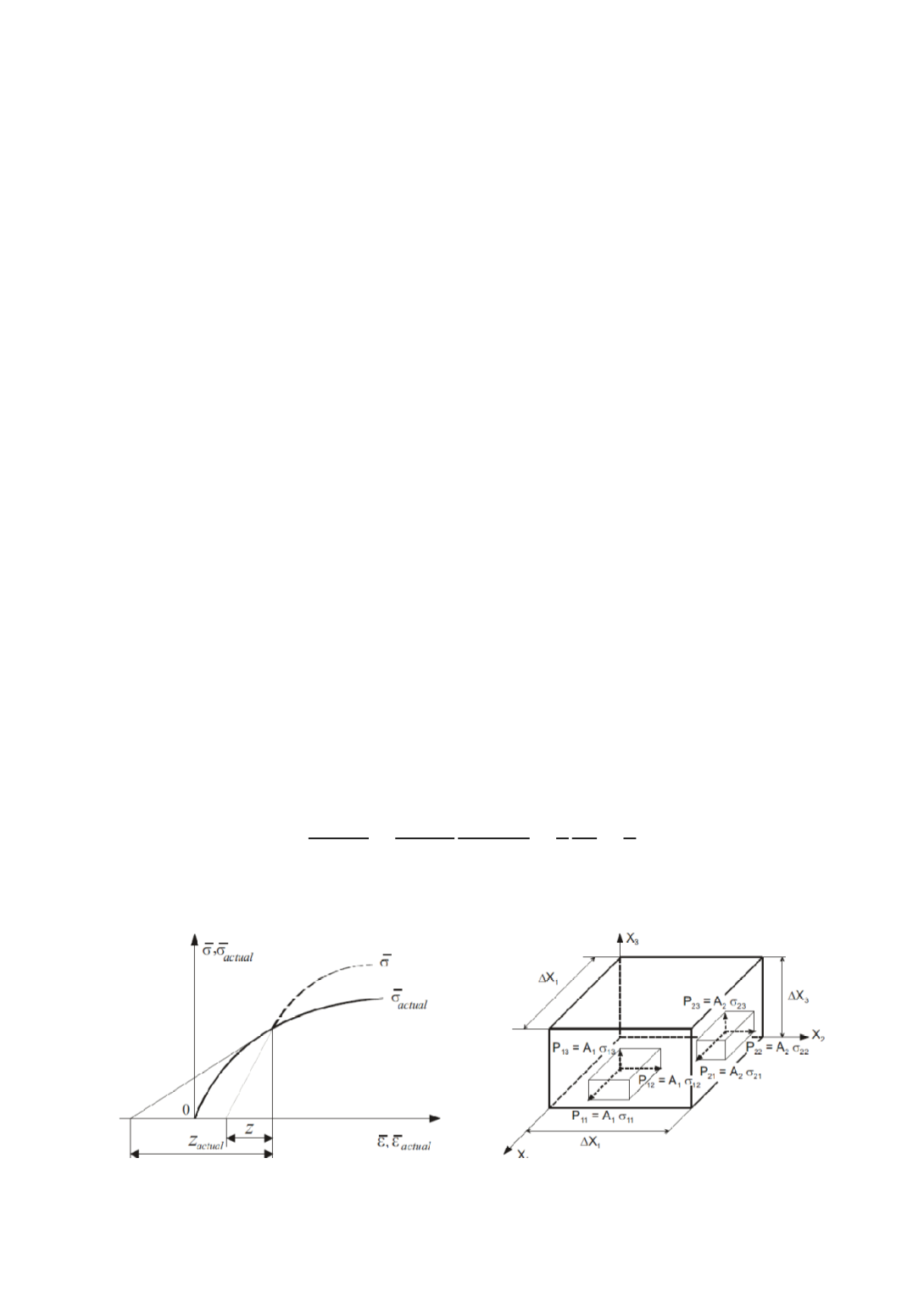
The limiting value of Z where this becomes equality is referred to as the critical
subtangent (Fig. 2.a).
(a)Definition (b) Hiller’s calculation of critical subtangent
Figure 2: Notion of critical subtangent